Multi-angle polarization simulations

POLDER is a wide field of view imaging radiometer that has provided the first global, systematic measurements of spectral, directional and polarized characteristics of the solar radiation reflected by the Earth/atmosphere system. Its original observation capabilities have opened up new perspectives for discriminating the radiation scattered in the atmosphere from the radiation actually reflected by the surface. The technical details of the instrument can be found here.

In order to switch on polarization with mystic, the following lines need to be included in the input file:

rte_solver mystic
mc_polarisation

The Rayleigh phase matrix is calculated based on the depolarisation factor of the parameterization by Bodhaine, 1999.

Land surface reflection is currently approximated by a Lambertian reflector, which per definition does not change the state of polarisation. To set the surface albedo just type

 albedo 0.2

Water surfaces strongly polarize in the region of the sun glint, in order to account for this effect, the parameterization by Tsang (FORTRAN code by Mishchenko available here) has been implemented. In order to include an ocean BRDF you may use

 bpdf_tsang u10 2

In this case the wind speed is set to 2 m/s.

For aerosol simulation pre-calculated phase matrices for the OPAC aerosol types are available, a typical desert aerosol can be specified as follows:

aerosol_default
aerosol_species_file desert

Water cloud phase matrices are also available, they can be included using

wc_file 1D wc.dat
wc_properties mie interpolate  

The pre-calculated aerosol and water cloud optical properties including phase matrices where generated using the mie tool in libRadtran. If you want to perform simulations for specific size distributions or refractive indices you may easily calculate the corresponding optical properties using the mie tool and use the output directly for uvspec simulations.

For ice clouds one parameterization is available: HEY (Hong, Emde, Yang) is based on single scattering properties calculated by Hong Gang, who used the programs by Ping Yang. I have then integrated this data over gamma size distributions to obtain optical properties for various effective radii. The HEY parameterization is available for various habits, e.g.

ic_file 1D ic.dat
ic_properties hey interpolate
ic_habit solid_column

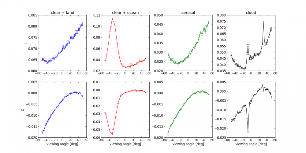
MYSTIC can not simulate various viewing directions at the same time, therefore it has to be called in a loop for multi-angle simulations. The python script below performs simulations at 443nm in the principal plane for four cases:

• clear sky atmosphere with Lambertian surface
• clear sky atmosphere with ocean surface
• atmosphere with typical desert aerosol
• atmosphere including a water cloud layer

The script directly plots the results:

All files needed to run this example are included in the following tgz-file: polarization_example.tar.gz

run_polarization.py

from pylab import *
import os
 
# Define input parameters
 
# case 0: Clear atmosphere with land surface (Lambertian)
# case 1: Clear atmosphere with ocean surface 
# case 2: Aerosol (desert)
# case 3: Water cloud (optical thickness 2)
ncases=4
cases=[0,1,2,3]
 
# Viewing angle
va=arange(-50., 1., 2., dtype='d')
umu=cos(va*pi/180.)
 
# Solar zenith angles
sza=[30.]
 
# Relative azimuth angles
phi=[0., 180.]
 
# wavelengths
lam=[443]
 
# Number of Stokes components
nstokes=4
 
# Number of photons
N = 1e4
 
# Initialize variables for radiance and standard deviation
radiance = zeros((len(va), len(sza), len(phi), len(lam), nstokes, ncases))
std = zeros((len(va), len(sza), len(phi), len(lam), nstokes, ncases))
 
# Path to uvspec executable
path=''
 
# Run RT calculation, set to false if you only want to modify the plots 
run_rt=True
 
if(run_rt):
    # Loop over all input parameters
    for case in cases:
        for ilam in range(len(lam)):
            for iphi in range(len(phi)):
                for isza in range(len(sza)):
                    for iumu in range(len(umu)):
 
                        disp('run mystic: lam %g phi0 %g sza %g va %.2f case %d'%(lam[ilam], phi[iphi], sza[isza], 
                                                                                  (arccos(-umu[iumu])*180./pi), case))
                        # mystic.inp: template file which includes settings that are not changed
                        tmp = open('mystic.inp').read()  
 
                        # mystic_run.inp: input file for uvspec, modified in the following 
                        inp = open('mystic_run.inp'%va[iumu], 'w')
                        inp.write(tmp)
                        inp.write('wavelength %g \n'%lam[ilam])
                        inp.write('umu %g \n'%umu[iumu])
                        inp.write('sza %g \n'%sza[isza])
                        inp.write('phi %g \n'%phi[iphi])
                        inp.write('mc_photons %d \n'%N)
                        if(case==0):
                            inp.write('albedo 0.2 \n') # Lambertian surface albedo of 0.2
                        elif(case==1):
                            inp.write('bpdf_tsang_u10 2 \n') # BPDF for ocean, wind speed 2
                        elif(case==2):
                            inp.write('aerosol_default \n')
                            inp.write('aerosol_species_file desert \n') # OPAC desert aerosol
                            inp.write('mc_vroom on \n') # switch on variance reduction for spiky phase functions
                        elif(case==3):
                            inp.write('wc_file 1D wc.dat \n')
                            inp.write('wc_properties mie interpolate \n')  
                            inp.write('wc_modify tau set 2 \n') # cloud optical thickness 2
                            inp.write('mc_vroom on \n') # switch on variance reduction for spiky phase functions
                        inp.close()
 
                        fin, fout=os.popen2(path+'uvspec < mystic_run.inp')
                        os.wait()
 
                        # Write Stokes vector and standard deviation into variables
                        # I
                        radiance[iumu,isza,iphi,ilam,0,case]=loadtxt('mc.rad.spc')[0,4]
                        std[iumu,isza,iphi,ilam,0,case]=loadtxt('mc.rad.std.spc')[0,4]
                        # Q
                        radiance[iumu,isza,iphi,ilam,1,case]=loadtxt('mc.rad.spc')[1,4]
                        std[iumu,isza,iphi,ilam,1,case]=loadtxt('mc.rad.std.spc'%va[iumu])[1,4]
                        # U
                        radiance[iumu,isza,iphi,ilam,2,case]=loadtxt('mc.rad.spc'%va[iumu])[2,4]
                        std[iumu,isza,iphi,ilam,2,case]=loadtxt('mc.rad.std.spc'%va[iumu])[2,4]
 
 
    np.save('radiance.npy', radiance)
    np.save('std.npy', std)
 
else:
    radiance=np.load('radiance.npy')
    std=np.load('std.npy')
 
# plot results 
figure(1, figsize=(16,8))
isza=0
ilam=0
 
colors=['b','r','g','k']
titles=['clear + land', 'clear + ocean', 'aerosol', 'cloud']
for case in range(ncases):
    subplot(2,4,case+1)
    errorbar(va, radiance[:,isza,0,ilam,0,case], std[:,isza,0,ilam,0,case], color=colors[case])
    errorbar(-va, radiance[:,isza,1,ilam,0,case], std[:,isza,1,ilam,0,case], color=colors[case])  
    title(titles[case])
    if(case==0):
        ylabel('I')
 
    subplot(2,4,case+5)
    errorbar(va, radiance[:,isza,0,ilam,1,case], std[:,isza,0,ilam,1,case], color=colors[case])
    errorbar(-va, radiance[:,isza,1,ilam,1,case], std[:,isza,1,ilam,1,case], color=colors[case])
    xlabel('viewing angle [deg]')
    if(case==0):
        ylabel('Q')
 
subplots_adjust(wspace=0.3)
 
savefig('polarization_example.png')